


Slow Start to Alaska Wildfire Season
Blame the weather

How slow a Start?
The 2023 Alaska wildfire season is off to a very slow start. As of June 18th the Alaska Interagency Coordination Center reports that just 1216 acres (492 ha) have burned in wildfires in Alaska to date in 2023. This is barely 1 percent of the median of the preceding 30 years. We have daily estimates of wildfire area burned since 19931 and this year is easily the least area burned in that time. In fact, only 2001 and 2008 had less than 10,000 aces (4000 ha) burned to June 18th. However, this is very hard to see in a conventional plot of area burned, such as in Fig. 1, due to the huge range of values (two orders of magnitude) and because, like many variables of interest in environmental sciences, there is a practical lower limit of zero, i.e. there can’t be less than zero area burned.
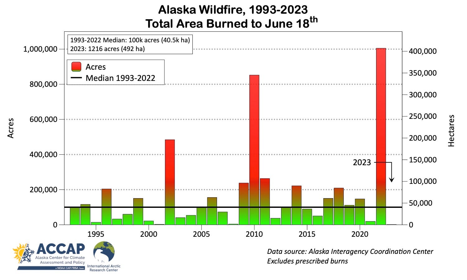
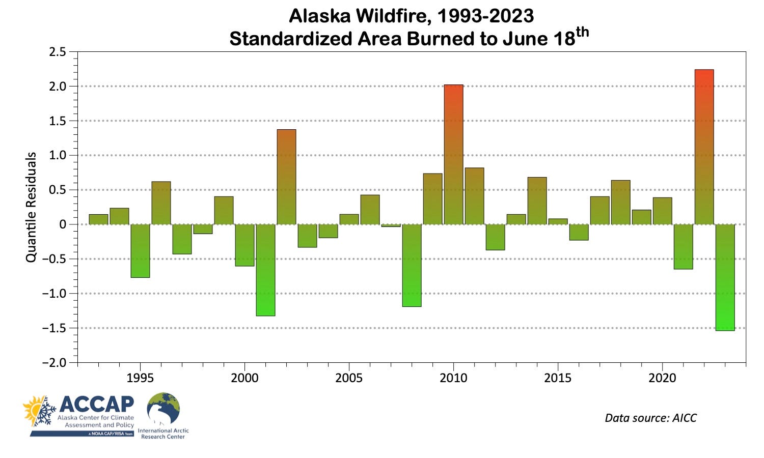
There are several oft-used techniques to get a better sense of variability in situations like this. One way is to use the logarithm of the variable of interest (in this case, area burned in wildfire). This can work if there are no actual zeros, but log plots take practice to interpret and can obscure details of interest. A method widely used in climate science is to express values in relation to some “normal”, usually a multi-decade mean or median. For variables like snowfall or precipitation, where “normal” can vary greatly, whether at a single place over the course of the year or at the same time but at different places, we regularly use “percent of normal”, though this can be problematic when/where “normal” is quite low and fails when “normal” is zero. Another method is to use rankings relative to a baseline period. For some climate variables where there isn’t a practical lower bound, such as temperature, we can scale the difference from normal by the typical variability via the standard deviation. This is known as standardized departures2 . Standardized departures work best when the distribution of the variable of interest is something like a “bell-shaped” curve and do not work well at all when there is a practical lower bound that overlaps the variability (early season wildfire acreage is a good example). The concept of standardized departures can be modified to address these issues by using “quantile residuals”. See the technical notes at the end of this post if you want to know more details and the citation, but if you’re familiar with standardized departures, you can think of quantile residuals as scaled standard deviations. The quantile residuals for Alaska wildfire to June 18th over the past 31 years are shown in Fig. 2: here we get an immediate sense of the relative differences each year that accounts for the very large range of the observed distribution of area burned and the zero lower limit.
Why so Little Wildfire?
So why has wildfire acreage been so low this year in Alaska? As always, wildfire activity in the North is largely determined by three factors: the susceptibility of vegetation to burn, the weather, and the spark to ignite fires. Over much of mainland Alaska, spring snowmelt was later than normal, so fuels started drying later than usual, though the impact of this factor is now fading into the past. By mid-June, current low wildfire is mostly due to the lack of sustained warm and dry weather and a lack of thunderstorms. Figure 3 shows the average state and wind flow of the middle atmosphere from late May through mid-June. The blue (cool) colors show areas with lower than average pressure aloft, while orange-red (warm) colors show areas with above average pressure.3 This pattern is not conducive to sustained warm early summer weather in Alaska, but rather favors considerable cloudiness and rain, though with average flow out of the south, in the primary Alaska wildfire area (the Interior), rainfall has mostly not be especially heavy. Without sustained warm dry weather, in general fires that start have much less opportunity to grow.
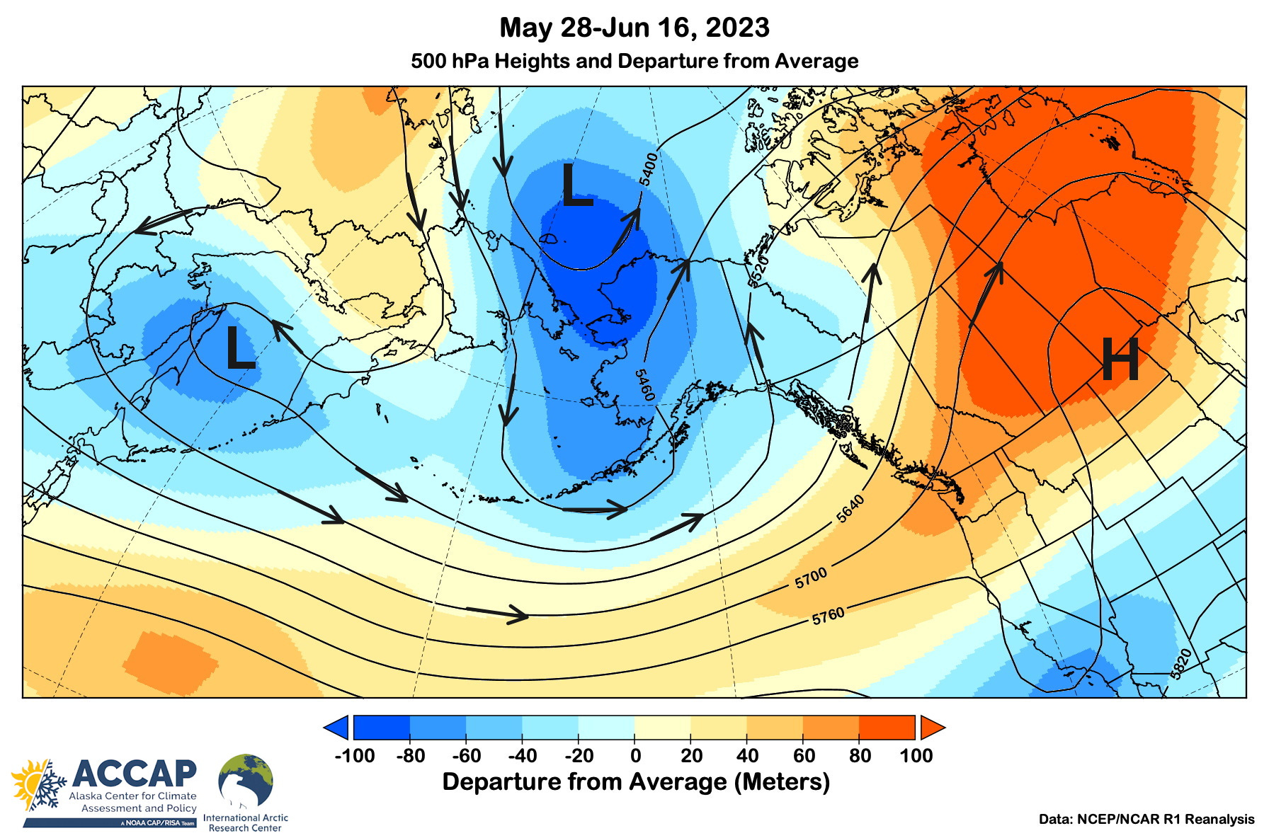
The “spark” factor has also been the very limited so far this summer, with much less thunderstorm activity than is typical. This is also tied to the mid-atmosphere pattern shown above. The low pressure and associated moisture and cool temperatures aloft are actually positive factors for thunderstorm development in Alaska. However, near-surface warmth is also needed this time of year and that has been lacking. Figure 4 plots the number of lightning strikes mid-May through June 17th each year since the current configuration of the Alaska Fire Service lightning detection network has been operational (since 2012). While there are only 12 years of observations, the only year with a similarly low number of strikes was 2013 (though the weather pattern that year was completely different than 2023).

While the clock is ticking on the Alaska 2023 wildfire season, it’s not over yet. However, fires that start after early July are much less likely to grow large. Nightime darkness gradually returns to Interior Alaska and overnight humidities tend to be higher resulting in shorter burn periods each day and most significantly, the climatological rainy season for Alaska begins in late July.
Technical details:
The Alaska Interagency Coordination Center is the first stop for all things wildfire-related in Alaska: https://fire.ak.blm.gov
Quantile residuals: “…general definition of residuals for regression models with independent responses. Our definition produces residuals which are exactly normal, apart from sampling variability in the estimated parameters, by inverting the fitted distribution function for each response value and finding the equivalent standard normal quantile.” From Dunn, P. K., & Smyth, G. K. (1996). Randomized quantile residuals. Journal of Computational and graphical statistics, 5(3), 236-244.
In Figure 2, quantile residuals computed using the R package “statmod”.
The Alaska Fire Service made near daily estimates of acreage burned prior to 1993 but so far no paper or electronic copies of the daily have surfaced. I keep hoping that someday someone will stumble upon a box with copies of the pre-1993 daily situation reports buried in a storage closet.
Standardize departures are easy to calculate: just the difference of the observed value minus “normal” over some baseline period divided by the standard deviation over the same baseline.
Technically of course, this is heights (in geopotential meters) since by construction the pressure is everywhere the same (500 hPa). That is an important but extremely technical meteorological point: for explanatory purposes here we can think of this as mid-atmosphere pressure without undo confusion.
Thanks Rick for these informative newsletters! Your insights are so valuable. Happy Solstice!